Part 2: Derivatives and Backpropagation — Making the Graph Learn

Part 2 of 3 in a code-first walkthrough of micrograd, based on Andrej Karpathy’s The spelled-out intro to neural networks and backpropagation.

In Part 1, we built a Value class that wraps floats and tracks how they were produced - a computation graph. But the graph alone doesn’t help us train anything. We need to know: if I nudge this input, how does the output change?

That question is answered by derivatives. This post adds gradient tracking and automatic backpropagation to the Value class.

Part 1: The Value class and forward pass
Part 2 (this post): Derivatives and backpropagation
Part 3: From engine to neural network

2.1 What Is a Derivative?

Concept: A derivative measures how sensitive a function’s output is to a small change in one of its inputs.

The numerical approximation:

df/dx ≈ (f(x + h) - f(x)) / h, where h is very small (e.g., 0.0001)

When a function has multiple inputs, we can measure sensitivity to each one separately by nudging that input while holding the others fixed.

Take the function:

f = a * b + c

with a = 2, b = -3, and c = 10. The current value of f is 2*(-3) + 10 = 4.

Nudging each input by 0.0001:

df/da ≈ ((2.0001 * -3 + 10) - (2 * -3 + 10)) / 0.0001 = -3.0

df/db ≈ ((2 * -2.9999 + 10) - (2 * -3 + 10)) / 0.0001 = 2.0

df/dc ≈ ((2 * -3 + 10.0001) - (2 * -3 + 10)) / 0.0001 = 1.0

What these numbers mean

df/da = -3 means nudging “a” up by a tiny amount makes f go down by about 3 times that amount.

df/db = 2 means nudging “b” up makes f go up by about twice that amount.

df/dc = 1 means f tracks “c” one-for-one: bump “c” up by a little, f goes up by the same little.

h = 0.0001

# derivative of f with respect to a
a = 2.0; b = -3.0; c = 10.0
f1 = a * b + c  # 4.0

a = 2.0 + h
f2 = a * b + c

print(f"df/da = {(f2 - f1) / h:.4f}")  # ≈ -3.0

2.2 The Chain Rule (Intuition)

Concept: If a variable “z” depends on variable “y”, and “y” depends on variable “x”, then:

dz/dx = dz/dy * dy/dx

If we take the below example:

z = 2y
y = 3x
dz/dx = dz/dy * dy/dx
dz/dx = 2 * 3 = 6

Analogy

If there is a bike that is moving twice the speed of a person and a car that is moving thrice the speed of the bike then the car is moving at 6 times the speed of the person. alt text

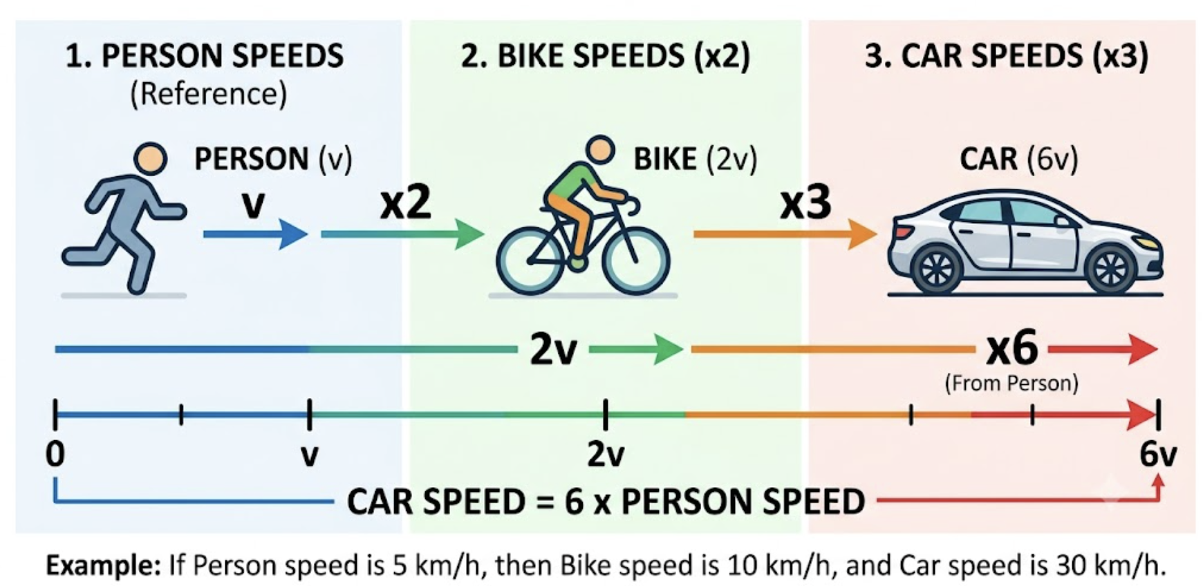
The above example is the essence of chain rule where we try to find out the answer that “How does my output change with respect to my input”? To figure out the relation between the speed of the person with respect to car we had to find all the intermediary relations and then multiply them to get our answer.

In a neural network there could be millions of these inputs/paramters therefore we would build methods in our value class that would assist us in finding local gradients

2.3 Storing Gradients

Concept: We now introduce a grad field on each Value. It will store the gradient of the final output with respect to that value — written as dL/d(self.data), where L is the loss (or whatever output we call .backward() on). We initialise it to 0.0, meaning “no gradient has been computed yet.”

Diff:


  class Value:
      def __init__(self, data, _children=(), _op=''):
          self.data = data
+         self.grad = 0.0
+         self._backward = lambda: None
          self._prev = set(_children)
          self._op = _op

Walkthrough:

self.grad = 0.0 is a single line, but it carries a lot of meaning:

What it stores. After backpropagation runs, v.grad will hold dL/dv — how much the final output changes for a tiny increase in v. This is the number we computed manually in section 2.1 using the numerical approximation.
Why 0.0 as the default. Before backpropagation runs, no gradient has been computed. Zero is the neutral starting value — it means “this value currently has no known effect on the output.”
Why this field matters for training. For leaf nodes — the weights and biases of a neural network — grad is ultimately what we care about. Once backpropagation has run, each weight’s .grad tells us the direction to nudge it to reduce the loss. That is the whole point of backpropagation.

We also set self._backward = lambda: None — a placeholder backward pass that does nothing. Each operation we implement next (__add__, __mul__, __pow__) will replace this with its own _backward function that knows how to push gradients to its inputs. Values that aren’t produced by an operation keep this default — we’ll see why that matters in section 2.7.

2.4 Backpropagation Through Addition

Concept:

When we compute L = a + b, we want to know: if the output L has some incoming gradient G, how much of that gradient flows back to a and b?

The local derivative of addition is straightforward:

d(a + b)/da = 1
d(a + b)/db = 1

Both derivatives are 1 — addition doesn’t scale or distort anything, it just passes values through. Applying the chain rule:

a.grad += G × 1 = G
b.grad += G × 1 = G

Addition is a gradient distributor. Whatever gradient arrives at the output, both inputs receive exactly that same gradient unchanged. This is the simplest possible backward pass.

Diff:


      def __add__(self, other):
          other = other if isinstance(other, Value) else Value(other)
          out = Value(self.data + other.data, (self, other), '+')
+         def _backward():
+             self.grad += out.grad
+             other.grad += out.grad
+         out._backward = _backward
          return out

Walkthrough:

_backward is a function stored on the output node. It won’t run immediately — it gets called later, during the backward pass, once out.grad is already known. At that point, it takes out.grad (the gradient flowing in from downstream) and distributes it back to the inputs.
Why both inputs get out.grad. This follows directly from the concept above: the local derivative of addition is 1 for both inputs, so the incoming gradient passes through unchanged.
Why += and not =. A value can appear more than once in an expression — for example, c = a + a. In that case, _backward would write to a.grad twice: once for the left input, once for the right. Using += lets both contributions accumulate to the correct total. Using = would overwrite the first contribution and give the wrong answer.

2.5 Backpropagation Through Multiplication

Concept:

When we compute c = a * b, the local derivatives are:

dc/da = b
dc/db = a

Intuitively: nudging a up by a tiny amount while holding b fixed changes the output by b times that amount. The bigger b is, the more sensitive c is to changes in a. The same logic applies in reverse for b.

Each input’s gradient is the other input’s value, scaled by the incoming gradient G:

a.grad += b * G
b.grad += a * G

This is the chain rule in action: local derivative × gradient from downstream.

Diff:


      def __mul__(self, other):
          other = other if isinstance(other, Value) else Value(other)
          out = Value(self.data * other.data, (self, other), '*')
+         def _backward():
+             self.grad += other.data * out.grad
+             other.grad += self.data * out.grad
+         out._backward = _backward
          return out

Walkthrough:

Let’s verify this numerically using the same approach from section 2.1 — nudging each input by a tiny amount and measuring how the output changes.

h = 0.0001
a = 2.0
b = -3.0

c1 = a * b  # baseline: -6.0

# nudge a, hold b fixed
c2 = (a + h) * b
print(f"dc/da ≈ {(c2 - c1) / h:.4f}")  # ≈ -3.0  (which is b)

# nudge b, hold a fixed
c2 = a * (b + h)
print(f"dc/db ≈ {(c2 - c1) / h:.4f}")  # ≈  2.0  (which is a)

Output:

dc/da ≈ -3.0000
dc/db ≈  2.0000

Nudging a by a tiny amount changed the output by -3.0 times that amount — exactly b. Nudging b changed the output by 2.0 times — exactly a. This confirms the local derivatives and gives us confidence that _backward is correct.

2.6 Backpropagation Through Power

Concept:

We can build intuition for the power rule directly from multiplication. Consider c = a², which is just a * a. From section 2.5, each input to a multiplication gets the other input’s value as its gradient. But here both inputs are the same a, so both contributions write to a.grad and accumulate:

a.grad += a * G   # from left input
a.grad += a * G   # from right input
─────────────────
a.grad  = 2a * G

The general rule follows the same pattern — c = a^n has derivative:

dc/da = n * a^(n-1)

This holds for negative powers too. The formula doesn’t change — only the sign and magnitude do. For example, with n = -1:

d(a^-1)/da = -1 * a^(-2) = -1/a²

Diff:


      def __pow__(self, other):
          assert isinstance(other, (int, float))
          out = Value(self.data ** other, (self,), f'**{other}')
+         def _backward():
+             self.grad += other * (self.data ** (other - 1)) * out.grad
+         out._backward = _backward
          return out

Walkthrough: We can verify both cases numerically:

h = 0.0001

# positive power: c = a^3
a = 2.0
c1 = a ** 3
c2 = (a + h) ** 3
print(f"dc/da ≈ {(c2 - c1) / h:.4f}")  # ≈ 12.0  (which is 3 * 2² = 12)

# negative power: c = a^-1
c1 = a ** -1
c2 = (a + h) ** -1
print(f"dc/da ≈ {(c2 - c1) / h:.4f}")  # ≈ -0.25  (which is -1 * 2^(-2) = -0.25)

Output:

dc/da ≈ 12.0000
dc/da ≈ -0.2500

2.7 The `backward()` Method — Topological Sort

Concept:

We have built _backward for each operation, but nothing calls them automatically. We need to call them ourselves — and in the right order.

The order is forced by how _backward works: every _backward reads out.grad to compute its inputs’ gradients. That means a node’s output must have its gradient set before we run that node’s _backward. In other words, we must always process a node before the nodes it feeds into — starting at the output and working backwards toward the inputs.

Take this example:

c = a + b
d = 2 * c
L = c + d

The correct order is:

L → d → c → a, b

We start at L (the output), then d (which feeds into L), then c (which feeds into both L and d), and finally a and b. Running them in any other order risks reading a gradient that hasn’t been set yet.

Topological sort is the algorithm that finds this ordering automatically for any computation graph.

Diff:


+     def backward(self):
+         topo = []
+         visited = set()
+         def build_topo(v):
+             if v not in visited:
+                 visited.add(v)
+                 for child in v._prev:
+                     build_topo(child)
+                 topo.append(v)
+         build_topo(self)
+
+         self.grad = 1.0
+         for node in reversed(topo):
+             node._backward()

Walkthrough:

The sort is built in the forward direction, then reversed for the backward pass. Here is how each piece fits together:

visited is a set that tracks which nodes have already been processed. It prevents the same node from being added to topo twice — important when a value is reused in multiple operations.
build_topo starts at the output node and recurses into its children before appending itself. This means a node is only added to topo after all the nodes it depends on have been added. The result is topo ordered leaves-first, output-last — the same direction as the forward pass.
reversed(topo) flips that order to output-first, leaves-last. This is the order we need for backpropagation: each node’s gradient is ready before its inputs’ _backward runs.
self.grad = 1.0 seeds the process. The derivative of the output with respect to itself is always 1 — this is what gets the chain rule started.
The loop calls node._backward() on every node, leaves included. This is where the self._backward = lambda: None default from section 2.3 earns its place. Leaf nodes — raw inputs like Value(2.0) — are never produced by an operation, so they never get a real _backward assigned. Without the no-op default, calling _backward() on a leaf would raise AttributeError. The placeholder lets the loop treat every node uniformly: leaves simply do nothing, since they have no inputs to pass a gradient to.

Tracing through the earlier example (L = c + d, d = 2 * c, c = a + b):

build_topo visits:   a, b, c, d, L   (leaves first)
topo stores:         [a, b, c, d, L]
reversed(topo):      [L, d, c, b, a]
_backward called in: L → d → c → b → a  ✓

Try it:

a = Value(2.0)
b = Value(-3.0)
c = Value(10.0)
d = a * b + c       # d = 4.0

d.backward()

print(a.grad)  # -3.0  — matches numerical derivative
print(b.grad)  #  2.0  — matches numerical derivative
print(c.grad)  #  1.0  — matches numerical derivative

2.8 The Complete Value Class (With Backpropagation)

import math

class Value:
    def __init__(self, data, _children=(), _op=''):
        self.data = data
        self.grad = 0.0
        self._prev = set(_children)
        self._op = _op
        self._backward = lambda: None

    def __repr__(self):
        return f"Value(data={self.data})"

    def __add__(self, other):
        other = other if isinstance(other, Value) else Value(other)
        out = Value(self.data + other.data, (self, other), '+')
        def _backward():
            self.grad += out.grad
            other.grad += out.grad
        out._backward = _backward
        return out

    def __mul__(self, other):
        other = other if isinstance(other, Value) else Value(other)
        out = Value(self.data * other.data, (self, other), '*')
        def _backward():
            self.grad += other.data * out.grad
            other.grad += self.data * out.grad
        out._backward = _backward
        return out

    def __pow__(self, other):
        assert isinstance(other, (int, float))
        out = Value(self.data ** other, (self,), f'**{other}')
        def _backward():
            self.grad += other * (self.data ** (other - 1)) * out.grad
        out._backward = _backward
        return out

    def __neg__(self):
        return self * -1

    def __sub__(self, other):
        return self + (-other)

    def __truediv__(self, other):
        return self * other**-1

    def __radd__(self, other):
        return self + other

    def __rmul__(self, other):
        return self * other

    def backward(self):
        topo = []
        visited = set()
        def build_topo(v):
            if v not in visited:
                visited.add(v)
                for child in v._prev:
                    build_topo(child)
                topo.append(v)
        build_topo(self)

        self.grad = 1.0
        for node in reversed(topo):
            node._backward()

Recap

In this post we taught the Value class to compute gradients:

Derivatives measure how sensitive an output is to a small nudge in each input (2.1).
The chain rule lets us combine local derivatives along a path by multiplying them (2.2).
We added a grad field to store each value’s gradient, and a _backward function on every operation that pushes gradients to its inputs — for addition, multiplication, and power (2.3–2.6).
backward() ties it together: a topological sort runs every node’s _backward in the right order, filling in grad across the whole graph from a single call (2.7).

The result is a complete autograd engine (2.8) whose gradients match the numerical estimates we started with.

What’s Next

The autograd engine is complete. Given any expression built from Value objects, you can call .backward() on the output and get the derivative with respect to every input — automatically.

But an engine alone isn’t a neural network. In Part 3, we’ll use this engine to build neurons, layers, and a full multi-layer perceptron, then train it on data using gradient descent.

Previous: Part 1 — The Computation Graph ← Next: Part 3 — From Engine to Neural Network →

Part 2: Derivatives and Backpropagation — Making the Graph Learn#

2.1 What Is a Derivative?#

2.2 The Chain Rule (Intuition)#

2.3 Storing Gradients#

2.4 Backpropagation Through Addition#

2.5 Backpropagation Through Multiplication#

2.6 Backpropagation Through Power#

2.7 The backward() Method — Topological Sort#

2.8 The Complete Value Class (With Backpropagation)#

Recap#

What’s Next#

Part 2: Derivatives and Backpropagation — Making the Graph Learn

2.1 What Is a Derivative?

2.2 The Chain Rule (Intuition)

2.3 Storing Gradients

2.4 Backpropagation Through Addition

2.5 Backpropagation Through Multiplication

2.6 Backpropagation Through Power

2.7 The `backward()` Method — Topological Sort

2.8 The Complete Value Class (With Backpropagation)

Recap

What’s Next