Understanding Neural Networks Part 1

Building a Neural Network Engine from Scratch Part 1: Building the Computation Graph — The Value Class and Forward Pass

Part 1 of 3 in a code-first walkthrough of micrograd, based on Andrej Karpathy’s The spelled-out intro to neural networks and backpropagation.

To understand how LLMs work, one needs to understand neural networks, and to understand neural networks, one needs to understand backpropagation. When I started my journey of learning how LLMs work, I was quite intimidated as to where to start. Luckily, Andrej Karpathy has already created a YouTube series called Neural Networks: Zero to hero that also has a supplmentary repository called micrograd — a minimal but architecturally complete implementation of a neural network and an autograd engine. It operates on scalar values rather than tensors, but the mechanics are real: real backpropagation, real gradient descent.

This is Part 1 of a three-part series:

• Part 1 (this post): will cover the Value class and forward pass — how a computation graph gets built
• Part 2: Derivatives and backpropagation — how gradients flow backward through the graph
• Part 3: From engine to neural network — building neurons, layers, and a training loop

What is autograd?

Think of a neural network as a very complicated recipe with billions of ingredient quantities. Autograd is the system that tells you exactly how tweaking each ingredient amount affects how good the final dish tastes — automatically, after every attempt. In technical terms, for each parameter it calculates how much and in which direction it should change to reduce the error — these calculations are called gradients — and it does this automatically across the entire network.

In short, autograd is what makes large-scale neural network training feasible. It sits quietly underneath frameworks like PyTorch and is largely invisible to most users, but without it, modern deep learning — and by extension LLMs — wouldn’t exist in their current form.

How to read this series

Each section introduces a small addition to the codebase, shown as a git-style diff. The format:

1. Concept — a short explanation of the idea being implemented
2. Diff — the code change
3. Walkthrough — what the code does and why it matters
4. Try it — a runnable snippet to verify the behaviour

1.1 A Wrapper That Remembers

Concept: Before we can do any calculus, we need a data structure that tracks how values were produced. A Value object wraps a plain float and records which operation created it and from which operands. This is the foundation of the computation graph that backpropagation will later traverse.

Diff:

+ class Value:
+     def __init__(self, data: float, _children: tuple =(), _op: str = ''):
+         self.data = data
+         self._prev = set(_children)
+         self._op = _op
+
+     def __repr__(self) -> str:
+         return f"Value(data={self.data})"

Walkthrough: The constructor currently contains the following values:

• data: It is the scalar that would store the floating point value of a variable
• _prev: Stores the set of Value objects that produced the current value.
• _op: Stores the mathematical operations (like +,-, *)

The __repr__ method allows us to display a Value object in a human-readable format, so that we can understand the contents of an object when we use the print() function.

Try it:

a = Value(2.0)
b = Value(3.0)
print(a)        # Value(data=2.0)
print(a._prev)  # set() — no parents, this is a leaf
print(a._op)    # '' — no operation produced this

1.2 Addition (Building the Graph, One Operation at a Time)

Concept:

So far we have only given the Value object the ability to store values and display them. Now we will add the functionality so that we can do mathematical operations between two or more Value objects.

Diff:

  class Value:
      def __init__(self, data: float, _children: tuple =(), _op: str = ''):
          self.data = data
          self._prev = set(_children)
          self._op = _op

+     def __add__(self, other: Value) -> Value:
+         out = Value(self.data + other.data, (self, other), '+')
+         return out

Walkthrough:

The __add__ method provides us the ability to use the + operator between two objects. It is returning a new Value object that is adding the data for both self and data and it is also populating _prev and _op values.

Try it:

a = Value(2.0)
b = Value(3.0)
c = a + b
print(c)        # Value(data=5.0)
print(c._prev)  # {Value(data=2.0), Value(data=3.0)}
print(c._op)    # '+'

1.3 Multiplication

Concept:

Similar to addition the __mul__ provides us the ability to use the * operator between two objects.

Diff:

+     def __mul__(self, other: Value) -> Value:
+         out = Value(self.data * other.data, (self, other), '*')
+         return out

Walkthrough: Logically the method is identical to __add__. It uses the * operator instead of +.

Try it:

a = Value(2.0)
b = Value(-3.0)
c = Value(10.0)
d = a * b + c
print(d)        # Value(data=4.0)
print(d._op)    # '+' — d is the result of an addition
print(d._prev)  # the mul result and c

1.4 Visualising the Computation Graph

Concept: If we consider the below python code:

a = Value(2.0)
b = Value(-3.0)
c = Value(10.0)
d = a + b
e = d * c

The computation graph would look as below:

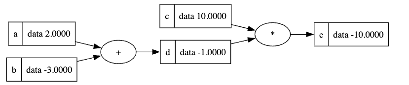
We can visually see how the variable d is related to a and b and how e is related to c and d. Considering that e is our final output that we want to increase or decrease as per our need, we will update the values of all the preceding nodes to achieve that.

1.5 More Operations: Power, Negation, Subtraction, Division

Concept: So far we have built the functionality of addition and multiplication. We can build negation, subtraction, and division on top of them. We will also introduce a __pow__ method that takes an integer or a float as the exponent and computes the result of exponentiation.

Diff:

+     def __pow__(self, other: int | float) -> Value:
+         assert isinstance(other, (int, float))
+         out = Value(self.data ** other, (self,), f'**{other}')
+         return out
+
+     def __neg__(self) -> Value:
+         return self * -1
+
+     def __sub__(self, other : Value) -> Value:
+         return self + (-other)
+
+     def __truediv__(self, other) -> Value:
+         return self * other**-1

Walkthrough:

One of the advantages of using the existing additon and multiplication functions is that we don’t have to pass the _children tuple in the initialiser.

Try it:

a = Value(4.0)
b = Value(2.0)
print((a - b).data)   # 2.0
print((a / b).data)    # 2.0
print((a ** 2).data)   # 16.0
print((-a).data)       # -4.0

1.6 Handling Raw Numbers (__radd__, __rmul__)

Concept: We need __radd__ and __rmul__ methods so that we can cater for equations like 2 + a or 2 * a. The current __mul__ and __add__ methods would fail as they expect to see an instance of Value object being passed to them.

Diff:

+     def __radd__(self, other: Value | float) -> Value:
+         return self + other
+
+     def __rmul__(self, other: Value | float) -> Value:
+         return self * other

After adding these 2 methods we also have to modify the existing __add__ and __mul__ methods so that they can cater for constant values

  def __add__(self, other: Value) -> Value:
+     other = other if isinstance(other, Value) else Value(other)
      out = Value(self.data + other.data, (self, other), '+')

  ...

  def __mul__(self, other):
+     other = other if isinstance(other, Value) else Value(other)
      out = Value(self.data * other.data, (self, other), '*')

Walkthrough:

With these two methods added we can now add or multiply constant values and now we can use equations like 2 * a + 1 or a + b - 3

Try it:

a = Value(3.0)
print((2 * a).data)    # 6.0  — triggers __rmul__
print((1 + a).data)    # 4.0  — triggers __radd__

1.7 The Complete Value Class (Forward Pass Only)

Now that we have added all the basic mathematical methods, our current Value class would look as shown below:

# Full Value class — forward pass only (no gradients yet)
from __future__ import annotations

class Value:
    def __init__(self, data: float, _children: tuple[Value, ...] = (), _op: str = '') -> None:
        self.data = data
        self._prev = set(_children)
        self._op = _op

    def __repr__(self) -> str:
        return f"Value(data={self.data})"

    def __add__(self, other: Value | float) -> Value:
        other = other if isinstance(other, Value) else Value(other)
        out = Value(self.data + other.data, (self, other), '+')
        return out

    def __mul__(self, other: Value | float) -> Value:
        other = other if isinstance(other, Value) else Value(other)
        out = Value(self.data * other.data, (self, other), '*')
        return out

    def __pow__(self, other: int | float) -> Value:
        assert isinstance(other, (int, float))
        out = Value(self.data ** other, (self,), f'**{other}')
        return out

    def __neg__(self) -> Value:
        return self * -1

    def __sub__(self, other: Value | float) -> Value:
        return self + (-other)

    def __truediv__(self, other: Value | float) -> Value:
        return self * other**-1

    def __radd__(self, other: Value | float) -> Value:
        return self + other

    def __rmul__(self, other: Value | float) -> Value:
        return self * other

What’s Next

At this point we have a Value class that can:

• Wrap any float
• Perform arithmetic (+, *, -, /, **)
• Track every operation in a computation graph

What it can’t do yet is tell us how changing any input affects the output. That’s the job of derivatives and backpropagation — the subject of Part 2.

Next: Part 2 — Derivatives and Backpropagation →